Isogeometric beam lattice
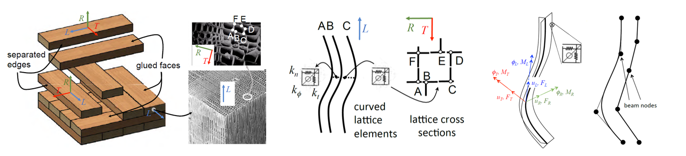
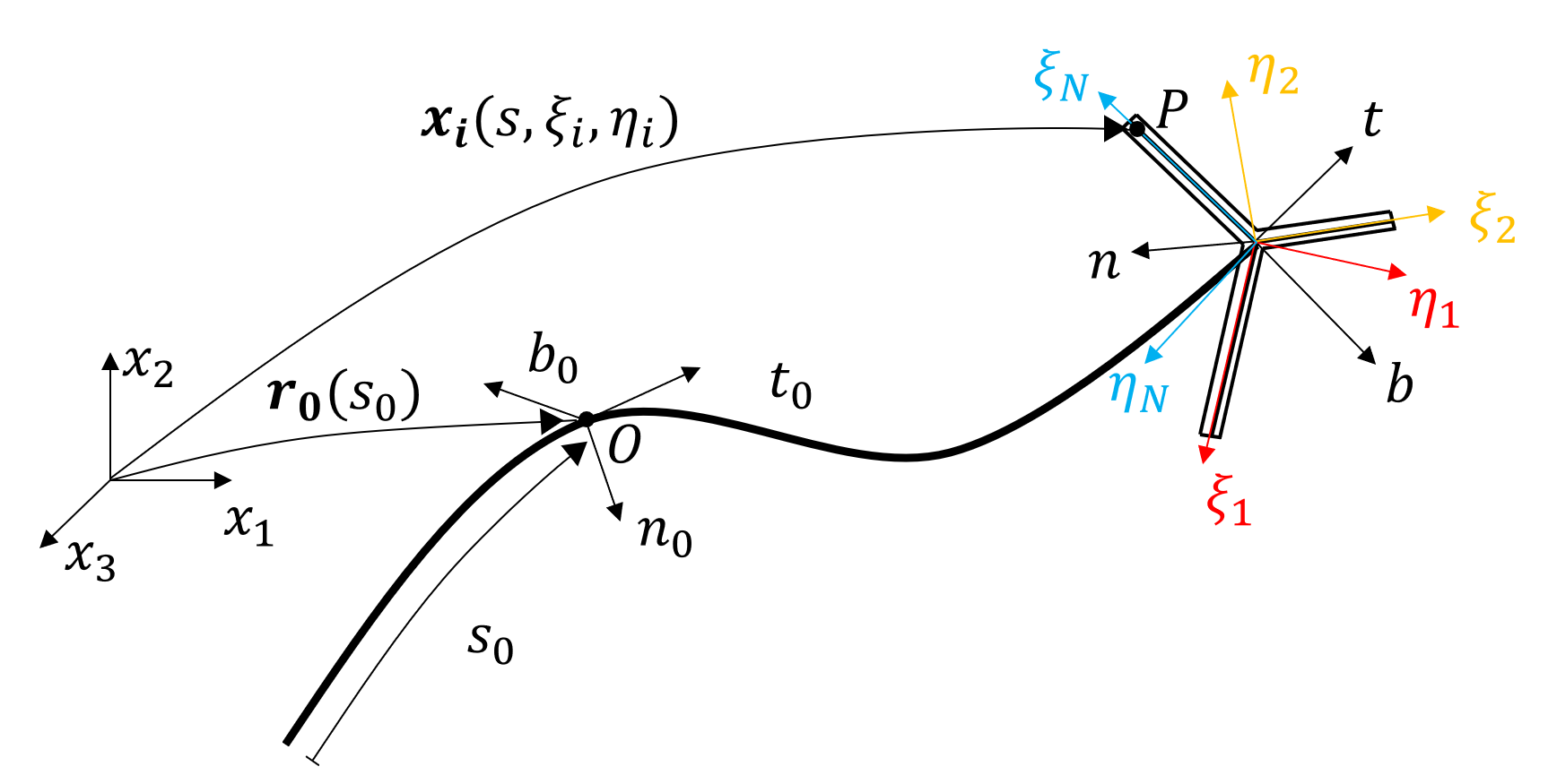
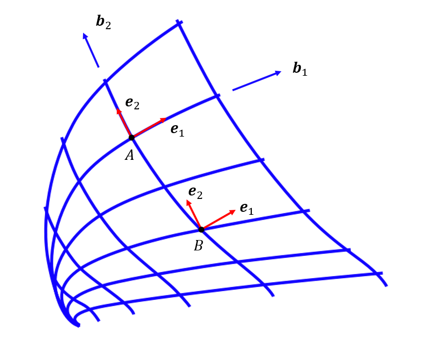
We approximate the internal structure of wood with a lattice system in which curved beam elements are located at the the common longitudinal sides shared by multiple cells (for examples, points A, B, C, D, E, and F in the figure below). The cross section of these beam elements is composed by portions of the cell walls attached to the shared edges. Each cell wall will be subdivided in two equal portions assigned to the two adjacent beams.
The beam behavior is governed by a newly derived Timoshenko beam formulation, which account for the geometrical curvature and torsion in 3D. The kinematic model of the beam was derived rigorously by adopting a parametric description of the axis of the beam, using the local Frenet–Serret reference system, and introducing the constraint of the beam cross ection planarity into the classical, first-order strain versus displacement relations for Cauchy' s continua. The resulting beam kinematic model includes a multiplicative term consisting of the inverse of the Jacobian of the beam axis curve. Its contribution vanishes exactly for straight beams and is negligible only for curved and twisted beams with slender geometry. Furthermore, to simplify the description of complex beam geometries, the governing equations were derived with reference to a generic position of the beam axis within the beam cross section.
Finally, this study pursued the numerical implementation of the curved beam formulation within the conceptual framework of isogeometric analysis, which allows the exact description of the beam geometry. This avoids stress locking issues and the corresponding convergence problems encountered when classical straight beam finite elements are used to discretize the geometry of curved and twisted beams.
Generalized formulation of 3D Timoshenko beams with irregular cross-sections
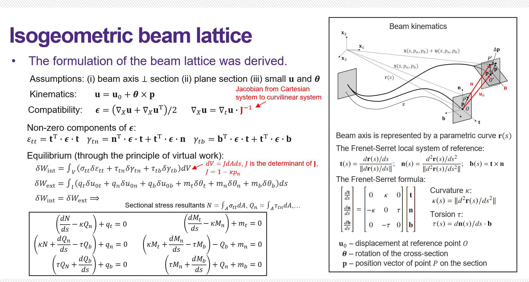
The underlying assumptions for the new beam formulation are the same as those made in classical Timoshenko beam theory: 1) the beam axis is orthogonal to the beam cross-sections before the deformation; 2) the cross-sections remain planar and preserve their shape and size during deformation; and 3) displacements and rotations are small compared to the beam size (first-order theory). The warping effects of the section planes are neglected in this work.
The geometry of a curved and twisted beam can be represented by a parametric curve of the beam axis $\mathbf{r}(s)$, as a function of the arc-length $s$, and a position vector on the cross-section $\mathbf{p}(p_{n},p_{b})$.
$$ \mathbf{x}(s,p_n,p_b) = \mathbf{r}(s) + p_n\mathbf{n}+ p_b\mathbf{b} $$
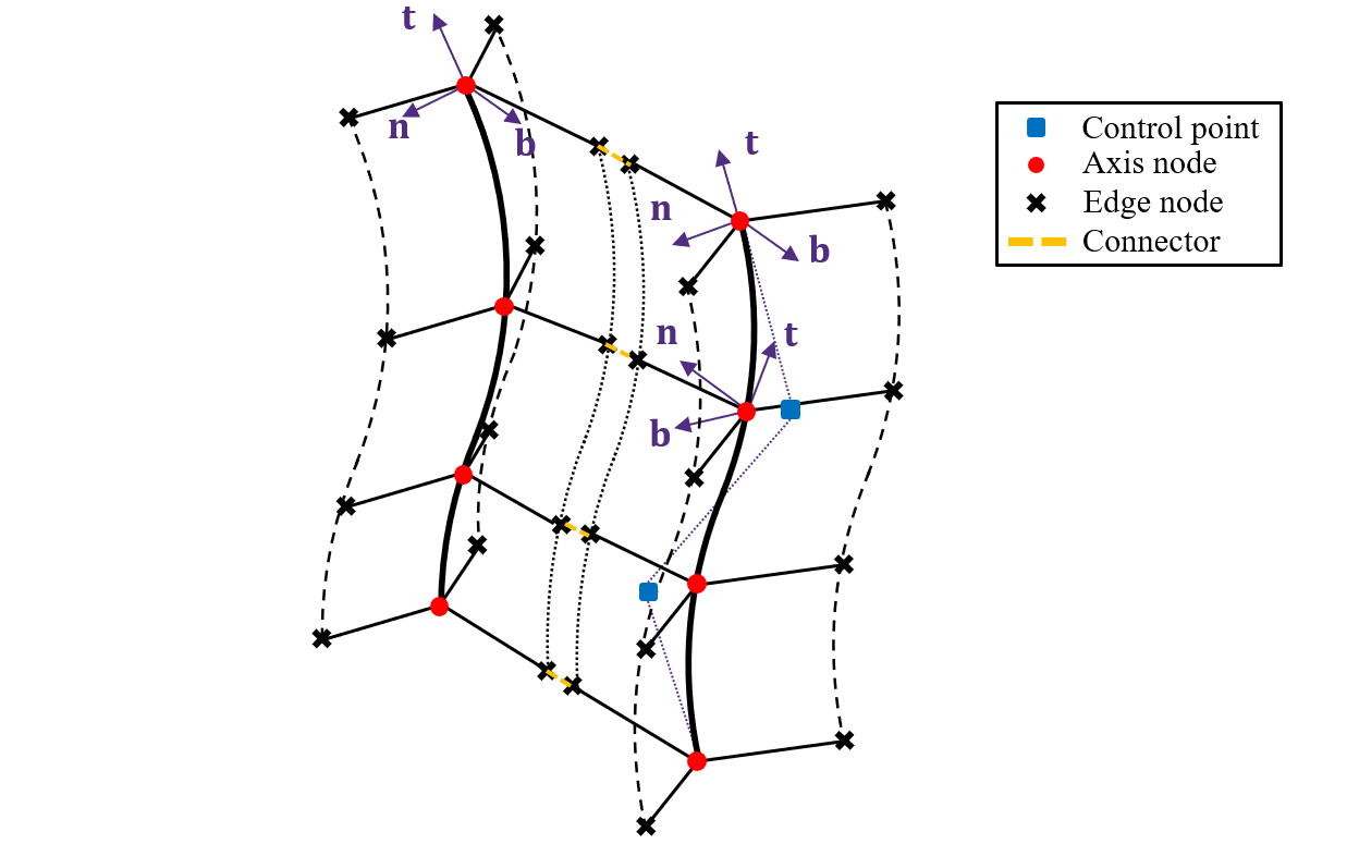
The vector $\mathbf{r}(s)$ allows calculating the Frenet-Serret local basis, as well as the local curvature $\kappa$ and torsion $\tau$, as shown in figure below:
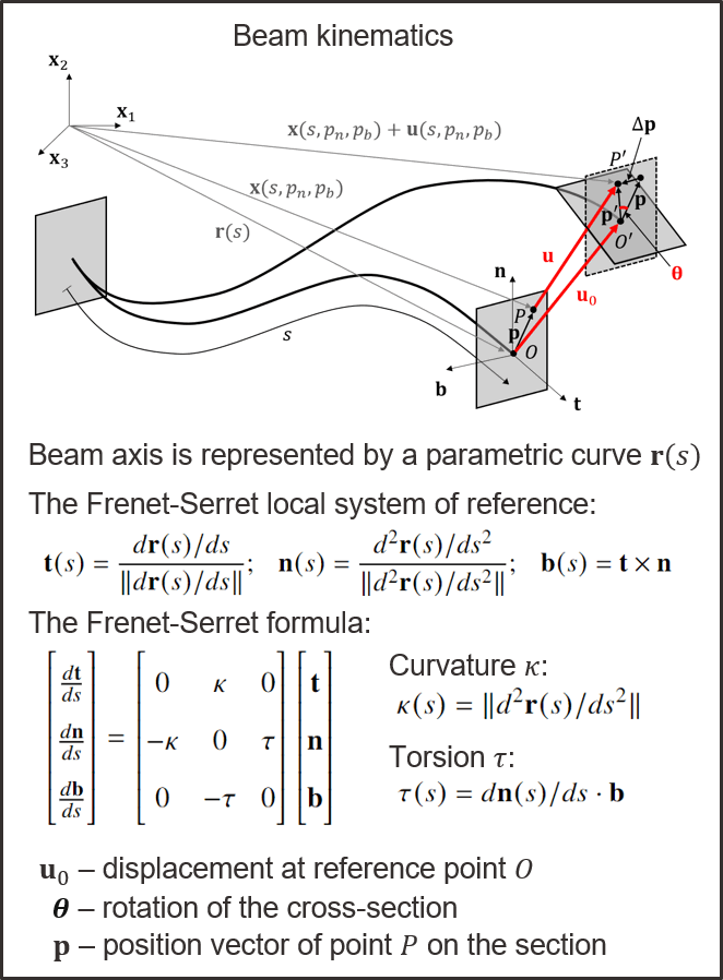
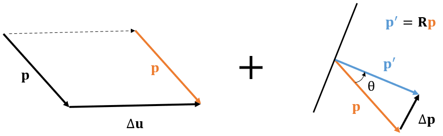
A generic point $\mathbf{x}$ can achieve a displacement vector $\mathbf{u} =\mathbf{u}(s,p_n,p_b)$, and this displacement can be decomposed into two parts: one is the displacement induced by rigid body translation of the cross section, another part is the displacement induced by the rigid body rotation of the cross section. For the rigid body rotation part, assume that the position vector of generic point after rotation $\mathbf{p}^{\prime}$, and the rotation matrix $\mathbf{R}$, according to Rodrigues' formula: $$ \mathbf{p'} = \mathbf{R}\mathbf{p} $$ where $$ \mathbf{R} = \mathbf{I}+(\sin{\theta})\mathbf{K}+(1-\cos{\theta})\mathbf{K}^2 ~~~~~~~~ \theta = | \boldsymbol{\theta}| $$
if the small rotation assumption applies, the displacement due to the rigid body rotation of the cross section $$ \mathbf{\Delta p} = \mathbf{p'}-\mathbf{p}= (\mathbf{R}-\mathbf{I})\mathbf{p}= [(\sin{\theta})\mathbf{K}+(1-\cos{\theta})\mathbf{K}^2]\mathbf{p}\approx \theta\mathbf{K}\mathbf{p} $$ one can further derive that $$ \theta\mathbf{K}\mathbf{p} = \boldsymbol{\theta} \times \mathbf{p} $$ hence the total displacement of a point at a generic point can be calculated as
$$\mathbf{u} = \mathbf{u}_0+\boldsymbol{\theta} \times \mathbf{p}$$
where $\mathbf{u}_0(s)$ is the cross-section translation, $\boldsymbol{\theta}(s)$ is the cross-section rotation with reference to point $O$ corresponding to the intersection between the axis and the cross-section. Point $O$ is any point in the cross-section and it does not need to be the cross-section centroid.
For the compatibility condition, note that the local Frenet-Serret coordinate ($t-n-b$) system is a curvilinear system, so we need to transform the displacement gradient $\nabla_{\mathbf{t}} \mathbf{u}$ back to the Cartesian system to use the small strain formula. The displacement gradient in the global reference system can be calculated as $\nabla_{\mathbf{X}} \mathbf{u}=\nabla_{\mathbf{t}} \mathbf{u} \cdot \mathbf{J}^{-1}$, where $\nabla_{\mathbf{t}} \mathbf{u}$ is the displacement gradient in the local system of reference and $\mathbf{J}$ is the Jacobian of the local to global transformation.
The small strain tensor in the global system of reference reads:
$$ \boldsymbol{\epsilon} = \frac{1}{2}\left(\nabla_{\mathbf{X}} \mathbf{u}+\nabla_{\mathbf{X}} \mathbf{u}^{\rm T}\right) $$
with non-zero components: one normal strain $\varepsilon_{tt} = \mathbf{t}^{\rm T}\cdot \boldsymbol{\epsilon}\cdot \mathbf{t}$, and two shear strains $\gamma_{tn} = \mathbf{n}^{\rm T}\cdot \boldsymbol{\epsilon}\cdot \mathbf{t}+\mathbf{t}^{\rm T}\cdot \boldsymbol{\epsilon}\cdot \mathbf{n}$, $\gamma_{tb} = \mathbf{b}^{\rm T}\cdot \boldsymbol{\epsilon}\cdot \mathbf{t}+\mathbf{t}^{\rm T}\cdot \boldsymbol{\epsilon}\cdot \mathbf{b}$. We can calculate and rewrite the non-zero components as a strain vector:
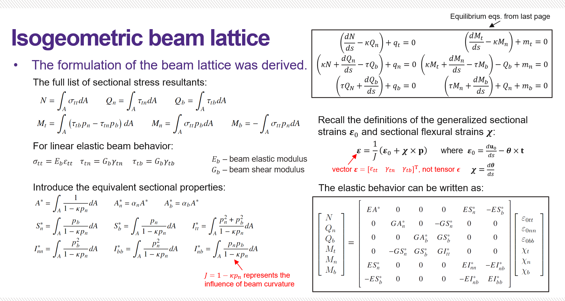
$$ \boldsymbol{\varepsilon} = \frac{1}{J}( \boldsymbol{\varepsilon}_0+\boldsymbol{\chi}\times\mathbf{p}) $$ where $\boldsymbol{\varepsilon}_0 = d\mathbf{u}_0/d s-\boldsymbol{\theta}\times\mathbf{t}$ is the generalized strain vector and $\boldsymbol{\chi}$ is the beam torsional/flexural curvature vector.
The above equation differs from the strain definition in classical Timoshenko beam formulations, which do not have the multiplier term $1/J=1/(1-\kappa p_n)$. An observation here is that the multiplier term is comprehensively governed by the local curvature $\kappa$ of beam axis, as well as by the cross-section size $p_n$ in the direction towards the curvature center. Hence this term is not negligible especially for highly curved, low-slenderness ratio (deep) beams.
The equilibrium of beam functions is somehow trivial, we followed the principle of virtual work to derive the governing equations of beam, the results are summarized in the figure below:
In linear elastic regime, we can write the stresses as $\sigma_{tt}=E\varepsilon_{tt}$, $\tau_{tn}=G\gamma_{tn}$, and $\tau_{tb}=G\gamma_{tb}$, where $E$ is the elastic modulus, $G=E/(2+2\nu)$ is the elastic shear modulus, and $\nu$ is Poisson's ratio.
In terms of stress resultants versus generalized strains and curvatures, the elastic behavior can be written as $\mathbf{f}=\mathbf{E}\boldsymbol{\eta}$. $\mathbf{f}=\left[N, Q_{n},Q_{b},M_{t},M_{n},M_{b} \right]^{\rm T}$ is the stress resultant vector, $\boldsymbol{\eta}=\left[\varepsilon_{0tt}, \gamma_{0tn},{\gamma_{0tb}},{\chi_{t}} ,{\chi_{n}},{\chi_{b}} \right]^{\rm T}$ is the generalized strain vector, $\mathbf{E}$ is the sectional stiffness matrix, as summarized in figure below:
Isogeometric analysis implementation of generalized Timoshenko beams
Isogeometric analysis (IGA) technique, populated by Hughes et al. in 2005, was used to accurately represent the geometry, and to alleviate the shear locking of curved beams during the analysis.
The IGA uses Non-Uniform Rational B-Splines (NURBS), which are originally used to represent the geometry in CAD industry, as shape functions to interpolate also the solution fields.
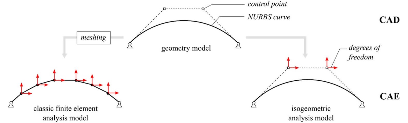
In the connector-beam lattice model (CBL), the beam wings that are respectively belonging to two neighboring beam lattice elements are inter-linked with cohesive connector elements, which will play an important role in the discrete aspect of the modeling. However, in IGA, the nodes that participate in the calculation are the control points, generally, they are not locating on the beam axis (see figure below).
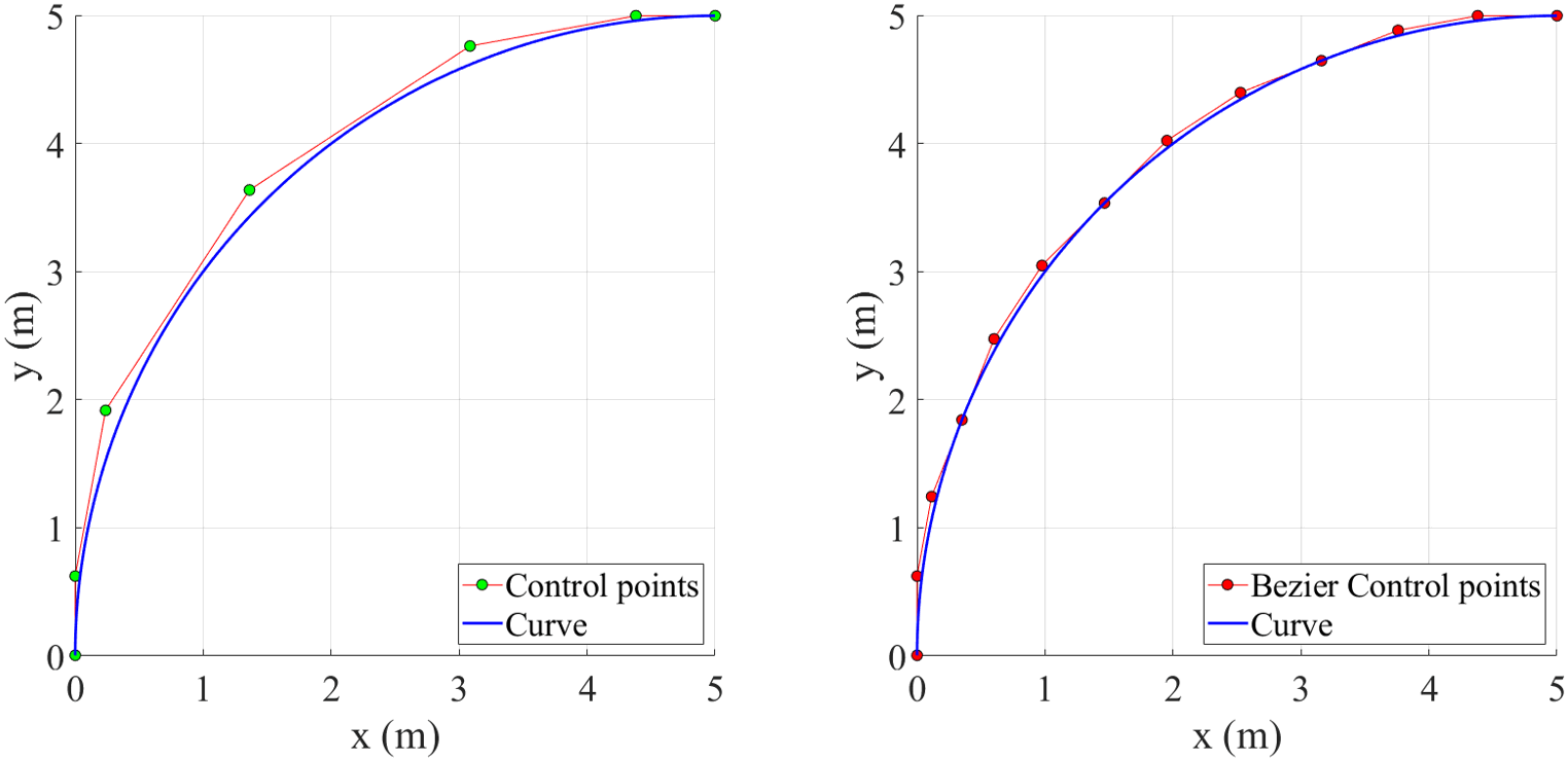
To having computational nodes on beam axis, we can map the field variables at the control points on the beam axis, or use another approach, called "Bézier Extraction".
The basic concept of IGA is discretizing the geometry and variable fields by the linear combination of the non-uniform rational basis splines (NURBS) control points and NURBS basis functions. A NURBS curve can be written as
$$ \mathbf{T}(\xi)=\sum_{A=1}^n R_A(\xi) \mathbf{P}_A=\mathbf{P}^{\mathrm{T}} \mathbf{R}(\xi) $$
where $\mathbf{R}(\xi)=\mathbf{W N}(\xi) / W(\xi), W(\xi)=\sum_{i=1}^n w_i N_i(\xi), \mathbf{W}$ is the NURBS weights matrix, $N(\xi)$ is the B-spline basis functions.
The corresponding Bézier curve is defined by
$$ \mathbf{T}(\xi)=\sum_{A=1}^{\mathrm{H}} B_A(\xi) \mathbf{P}_A^b=\left(\mathbf{P}^b\right)^{\mathbf{T}} \mathbf{B}(\xi) $$
where $\mathbf{B}(\xi)$ is the Bernstein polynomial basis functions. We can also rewrite the weight function $W(\xi)$ in terms of the Bernstein basis as
$$ W(\xi) =\mathbf{w}^{\mathrm{T}} \mathbf{N}(\xi) =\mathbf{w}^{\mathrm{T}} \mathbf{C B}(\xi)=\left(\mathbf{C}^{\mathrm{T}} \mathbf{w}\right)^{\mathrm{T}} \mathbf{B}(\xi)=\left(\mathbf{w}^{b}\right)^{\mathrm{T}} \mathbf{B}(\xi)=W^{b}(\xi) $$
The Bézier extraction operator is defined by:
$$ \mathbf{N}(\xi) = \mathbf{C}\mathbf{B}(\xi) $$
where $\mathbf{w}^{b}=\mathbf{C}^{\mathrm{T}} \mathbf{w}$ are the weights associated with the Bézier basis functions. The Bézier control points are now computed as
$$ \mathbf{P}^{b}=\left(\mathbf{W}^{b}\right)^{-1} \mathbf{C}^{\mathrm{T}} \mathbf{W} \mathbf{P} $$
This equation can be interpreted as mapping the original control points into projective space, applying the extraction operator to compute the control points of the projected Bézier elements, and then mapping these control points back from projective space.
Implementation of isogeometric beam lattice
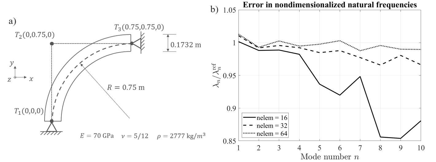
The isogeometric beam lattice elements have been implemented with Abaqus user subroutines "UEL" and "VUEL" for both implicit and explicit analyses. The numerical verification of beam lattice with varying cross-sectional properties has been performed, one example is shown in figure below:

IGA beam verification, free vibration: a) the model setup, b) ratio of simulated result $\lambda_n$ over the reference result $\lambda_n^{ref}$ for first 10 non-dimensionalized natural frequencies for a circular simply-supported beam (quadratic elements):
If you find this work useful, or if it helps you in your research on Timoshenko beam theory, we kindly ask that you cite this paper:
@article{yin2022generalized,
  title={Generalized Formulation for the Behavior of Geometrically Curved and Twisted Three-Dimensional Timoshenko Beams and Its Isogeometric Analysis Implementation},
  author={Yin, Hao and Lale, Erol and Cusatis, Gianluca},
  journal={Journal of Applied Mechanics},
  volume={89},
  number={7},
  pages={071003},
  year={2022},
  publisher={American Society of Mechanical Engineers}
}