The Connector-Beam Lattice Model for wood
Interest in engineered wood products (EWP) in construction industry is at a new high due to the low CO2 emission relative to structural properties and innovations of mass timber (e.g., gluelam, cross laminated timber). However, persistent issues stuck in front of the development of engineered wood products are the complex material behaviors of wood due to its inherent material anisotropy and heterogeneity, and consequently the reliance on extensive broad-based laboratory testing for the design and code approval of new products. To guide the laboratory testing and provide a computational tool to obtain data with high fidelity for the material properties of EWP, we propose a Connector-Beam Lattice Model for Wood (CBL-W) in 3D, which aims to naturally capture the morphological features of wood cellular micro-structure by using the connector-beam system, and to explicitly simulate the damages/cracks at the constituent material level by employing discrete-type cohesive fracture constitutive laws. The CBL-W model is a discrete-type model established on a morphologically-reproduced geometry of wood cellular structure at the microscale, and is calibrated and validated through a series of laboratory tests and mining of a vast database of wood product performance.
Model formulation
Isogeometric beam lattice
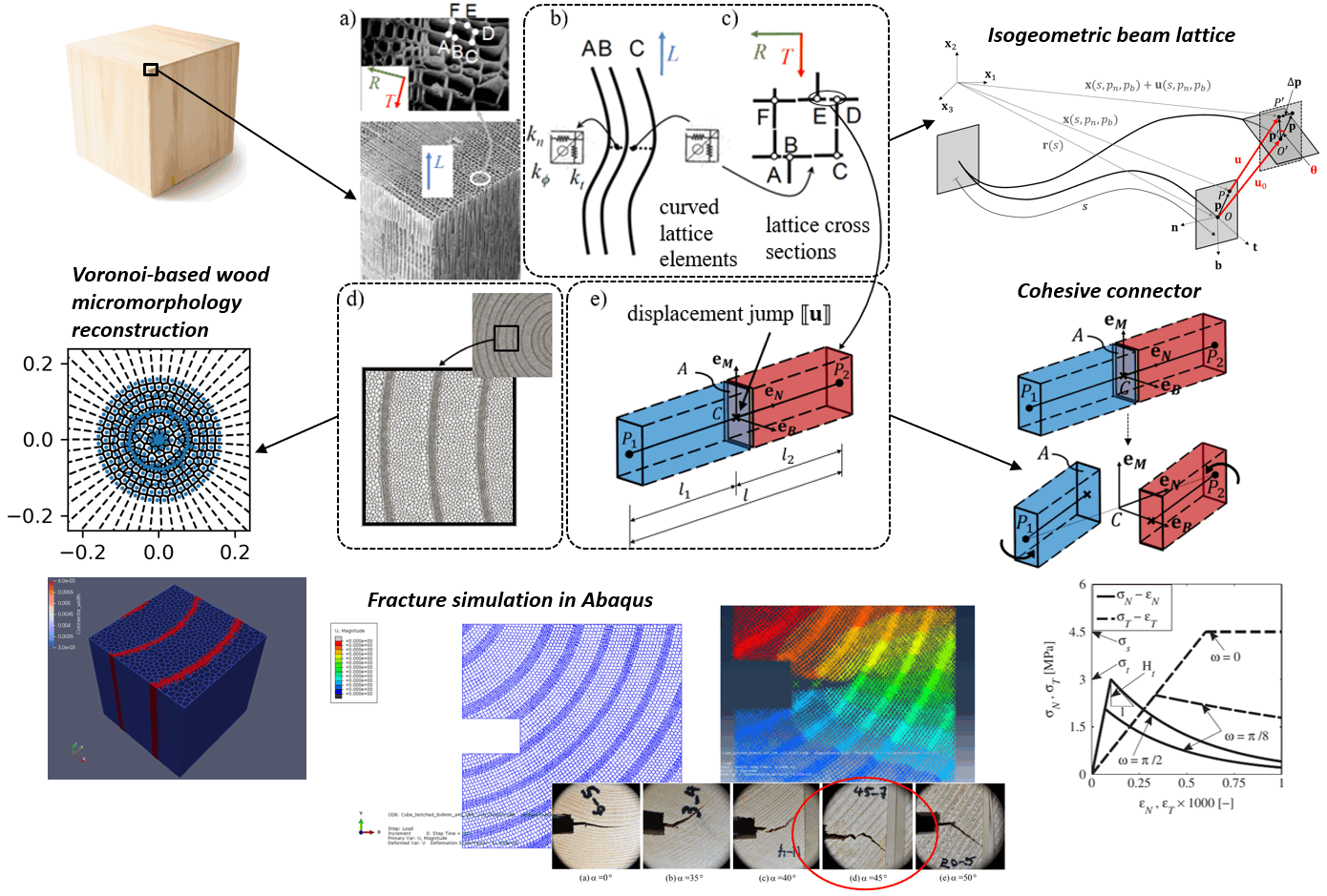
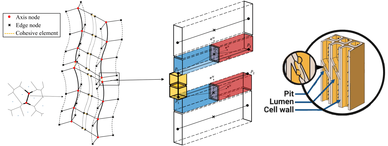
At the meso-scale, the morphology of softwood is characterized by a cellular structure in which each cell
has a straw-like appearance (see a and b in figure below). The cross section of each cell has approximately a polyhedral shape with, in the majority of
cases, 4-6 sides. We employ previously developed 3D curved beam elements, named isogeometric beam lattices, as shown in d) in figure below to capture the meso-scale morphology of wood cells. The beam lattices have varying, cruciform cross-sections. The thickness of the cell wall is not constant and it tends to be larger for latewood than
earlywood. Reflecting on the cross-sectional properties of beam lattices, the number of wings, the lengths and widths of wings vary in accordance with the wood morphology.
The length range of the beam lattices is 20-50 microns, depending on the wood species and the cell types of earlywood, latewood.

The detailed derivation, formulation and implementation of isogeometric beam lattice can be found in the page of Isogeometric beam lattice or in this paper.
Connector
Except the beam lattices, 1D nonlinear cohesive elements, named connectors, also exist in the model. They transversely and longitudinally connect pairs of adjacent beams, and account for the in-plane and longitudinal deformability of the cell walls which cannot be captured by the beam formulation.
Each connector element is substantially a 1D straight connecting-strut with length $l$ at the undeformed state (initial/total configuration), it connects a pair of "axis nodes" on the associated beam axes (red dots in figure below) in the lattice system.
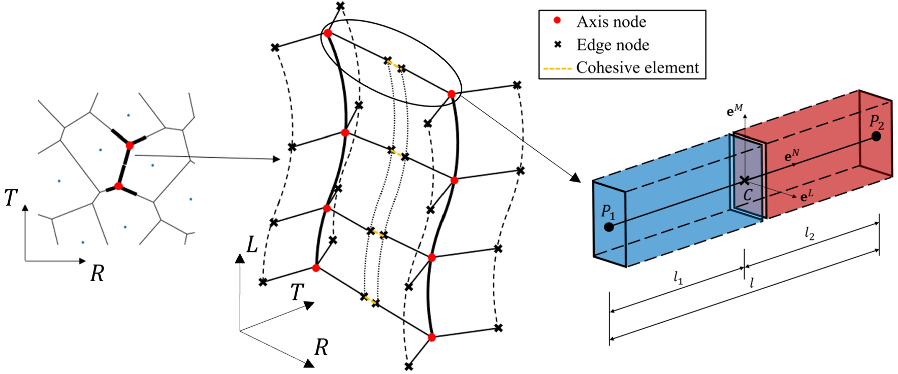
Each connector is assigned a constant cross-section $C$ that is corresponding to the joint surface of the cell wall. This surface is selected as the representitive failure surface. Once the system deforms, the two halves of the connector element move respectively and can separate, compress, and/or slide at the center-section $C$, which will lead to a displacement jump at the center-section.
This displacement jump can be idealized as an overall consequence of rigid-body motions of two halves of the connector element (two adjacent beams): $$ \llbracket \mathbf{u}_C \rrbracket = \mathbf{u}_C1 - \mathbf{u}_C2 $$
$$ \mathbf{u}_{C I}=\mathbf{u}_I+\boldsymbol{\theta}_I \times\left(\mathbf{x}_C-\mathbf{x}_I\right) \quad I \in 1,2 $$
where $\mathbf{x}_I$, $\mathbf{u}_I$, $\boldsymbol{\theta}_I$ are the nodal positions, displacements, and rotation angles at axis nodes $I \in 1,2$, respectively; $\mathbf{x}_C$ is the centroid position of center-section $C$.
For the computational simplicity in mathematical formulae for describing the fracture behaviors of wood cell walls, we employed a vectorial cohesive constitutive law, which was originally adopted in the microplane stress theory combined with the crack band model proposed by Bažant for the fracture/softening phenomena for quasi-brittle materials, including wood.
Our vectorial constitituve law requires the strain components in local normal and shear directions, which can be achieved by the projection of displacement jump at center-section $C$ onto local directions:
$$ \varepsilon_N=\mathbf{e}^N \cdot \llbracket \mathbf{u}_C \rrbracket / l \quad \varepsilon_M=\mathbf{e}^M \cdot \llbracket \mathbf{u}_C \rrbracket / l \quad \varepsilon_L=\mathbf{e}^L \cdot \llbracket \mathbf{u}_C \rrbracket / l $$
$\mathbf{e}^N$, $\mathbf{e}^M$, $\mathbf{e}^L$ are one normal and two tangential basis vectors for the connector element, respectively.
For elastic behaviors, linear relationship is assumed for both normal and tangential directions:
$$ \sigma_N=E_N \varepsilon_N \quad \sigma_M=E_T \varepsilon_M \quad \sigma_L=E_T \varepsilon_L $$
where, $E_N=E_0$, $E_T=\alpha E_0$, $E_0$ and $\alpha$ are effective normal modulus, shear-normal coupling parameter, respectively. $E_0$ and $\alpha$ are mesoscale material properties that can be identified from results of experimental tests in the elastic regime.
Regarding the nonlinear behaviors, for tension cases $(\varepsilon_N>0)$, the constitutive law satisfies the incremental elasticity condition:
$$ \dot{\sigma}=E_0 \dot{\varepsilon} \quad 0 \leq \sigma \leq \sigma_{b t} $$
where effective stress $\sigma =\sqrt{\sigma_N^2+\sigma_T^2 / \alpha}$, $\sigma_T=\sqrt{\sigma_M^2+\sigma_L^2}$, and effective strain $\varepsilon =\sqrt{\varepsilon_N^2+\alpha \varepsilon_T^2}$, $\varepsilon_T=\sqrt{\varepsilon_M^2+\varepsilon_L^2}$, these two thermodynamically consistent measures are selected.
The effective stress boundary $\sigma_{b t}(\varepsilon)$ is enforced through vertical return algorithm during iteration, it can be calculated by $\sigma_{b t}=\sigma_0 \exp \left(-H_0\left\langle\varepsilon-\varepsilon_0\right\rangle / \sigma_0\right)$, where $\sigma_0$ is the strength limit of effective stress, $\varepsilon_0=\sigma_0/E_0$ is the strain corresponding to the strength limit, $H_0$ is the softening modulus. The Macaulay bracket term $\langle x\rangle=\max [x, 0]$ reflects the irreversible strain-history dependence of $\sigma_{b t}$.
The strength limit of effective stress $\sigma_0$ is a function of direction of straining $\omega: \tan \omega=\alpha^{-1/2}\varepsilon_N/\varepsilon_T$, tensile strength $\sigma_t$, shear-normal strength ratio $r_{st}=\sigma_s/\sigma_t$, and shear-normal coupling parameter $\alpha$, i.e., $\sigma_0=\sigma_0\left(\omega,\sigma_t, r_{s t}, \alpha\right)$.
The softening modulus (post-peak slope) $H_0$ is a function of straining direction $\omega$:
$$ H_0=H_t\left(\frac{2 \omega}{\pi}\right)^{0.2} $$
For pure tension ($\omega=\pi/2$), $H_t$ is the post-peak slope calculated according to the energy dissipation during mesoscale damage localization (mode I fracture), which reads $H_t =2 E_0 /\left(l_t / l-1\right)$, where $l$ is the size of connector element, the characteristic length $l_t = 2 E_0 G_t / \sigma_t^2$ is derived in crack band model and represents the size of crack tip Fracture Process Zone (FPZ) of the quasi-brittle material, $G_t$ is the meso-scale fracture energy.
For pure shear ($\omega=0$), $H_0=0$, no softening and perfect plasticity is assumed.
Another type of connector also exists and can represent the weak joint (e.g., pit in the figure below) in the longitudinal direction. These longitudinal connectors have been considered in the model to permit the simulation of fiber rupture. Unlike the transverse connectors having cross-sectional properties of associated cell walls, the longitudinal connectors share the same cross-sectional properties with the associated beam elements.
Computational pipeline for wood simulations
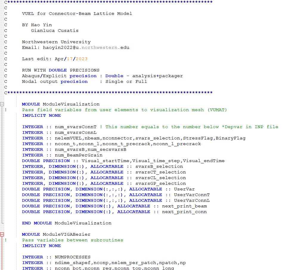
The beam lattice and connector elements have been implemented with Abaqus user subroutines UEL and VUEL for both implicit and explicit analyses. A preprocessing-analysis-postprocessing pipeline has been formed. The RingsPy package has the option to export the Abaqus .inp input files, which can be directly used for CBL-W simulations.
The post-processing of the CBL-W models can be directly achieved within Abaqus by employing the so-called "ghost mesh" or "phantom mesh". The post-processing is also implementated in a popular visualization tool Paraview. The isogeometric beam is visualized in Paraview with the Bezier curves.
|
|
|
|
The codes has been optimized for fast parallel computing for the large model simulations (number of elements > 10 millions). With the help of Northwestern's High-Performance Computing (HPC) Cluster - Quest, we are able to run large scale simulations with acceptable simulation times. The length scale of specimens can be up to tens centimeters as a mesoscale model with lattice element sizes of 10~100 microns.
In the video below, the specimen size in the simulation was around 5 cm x 5 cm x 2.5 cm (width x height x depth), totally 4 millions elements, and over 300,000 increments were involved. The simulation wall clock time was 55 hours with 64 CPUs (3rd Generation Intel(R) Xeon(R) processors).
Numerical simulations
Orthotropic Elasticity
Wood is often idealized as a homogeneous, orthotropic material in engineering practice. Based on the direction of wood grains, three principal orthogonal directions of elasticity for wood, i.e., longitudinal (L), tangential (T) and radial (R) are determined. Within elastic regime, because of the symmetry of mutually perpendicular planes and the relationship of Poisson's ratios $\nu_{ij}/E_{i}=\nu_{ji}/E_{j}$ (no sums), twelve independent elastic constants such as three elastic moduli, $E_L$, $E_T$, $E_R$, three transverse elastic moduli, $G_{TR}$, $G_{RL}$, $G_{LT}$, and six Poisson's ratios, $\nu_{T R}$, $\nu_{T L}$, $\nu_{R L}$, $\nu_{R T}$, $\nu_{L T}$, $\nu_{L R}$, are determined.

Under construction!
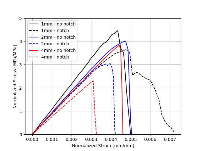
Size effect in transverse fracture
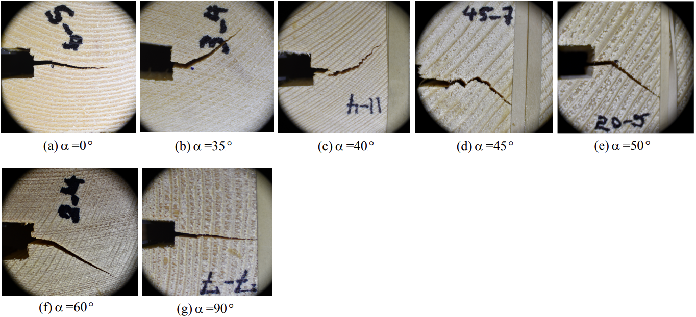
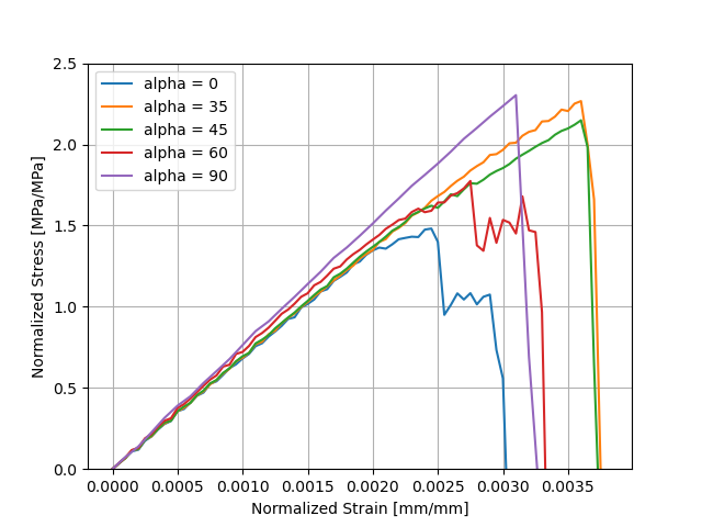
Growth ring orientation effects in transverse fracture